Excel Absolute and Relative Cell References and Autofill Function【Data Analysis Excel Skill】
You can learn the differences in Absolute and Relative Cell References with case study examples. Mastering Cell References increases your work speed greatly.
(Duration: 6:49)
<< Related Posts >>
- How to learn Excel functions, and a look at Excel functions: SUM, SUMIF and SUMIFS
- TEXT Function, which makes dates and numbers easily read and understood【Excel Skills】
The ‘Double-Click’ Method of Excel Autofill Function
Hi, this is Mike Negami, Lean Sigma Black Belt.
Today’s agenda is the AutoFill function and how to refer to other cells. These two features are essential when you do data analyses with Excel. Let’s start with the first one, Autofill.
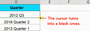
For example, in this worksheet, there is a purchase date column in Column A and formulas are contained in all the cells in Column D. If I had to type all of these manually, I would stop using Excel. Of course, this is not the case. When you change or type the formula in the top cell, you would like to apply that downwards. If you select a cell, the lower right corner of the cell becomes a small square. Hover your cursor over it, then the cursor turns into a black cross.

As you drag it down, the first formula will be copied. However, if there are many rows, it takes a lot of time. Instead, you can double-click when you see the cross, then you can copy it to the bottom in a flash. I was impressed when I first did it!
When you select an entire column and hover your cursor over the top right corner, your cursor turns into a black cross. Dragging it to the right will copy everything including the column width.
What’s Absolute and Relative Cell References?
But there is a problem. If you double-click a formula in Column D, you can see a blue color and that the formula is referring to a purchase date and calculates its fiscal quarter. However, in the copied Column E, the reference destination is shifted to the ‘Sales Channel’ in Column B and all the cells will be in error (See the image above). Here, you need to understand absolute and relative cell references. The words themselves are not important, but please understand the differences in the two aspects of that concept.
If we look at the formulas we copied downward earlier, the referencing cells are shifted downward too. Since you want to show each quarter next to each date, this is just fine. This reference method is ‘relatively shifted’, so it’s called the ‘Relative Reference’. However, there are times when you don’t want it to shift like the one we copied horizontally. In that case, we use ‘Absolute Reference’. It’s easy to do that, just enter a ‘$ (dollar)’ symbol.
In this example, since you want the reference to be fixed to Column A, meaning to make it absolute, put a ‘$ (dollar)’ symbol in front of A (See the image above). Then auto-fill the cell downward again and copy the column horizontally again. We don’t get any errors this time. Please be aware that the references are fixed horizontally, but they remain relative, vertically.
To summarize, when copying horizontally, the column letters would change. Instead, if you want them to be ‘absolute’, place the $ symbol in front of the letters. On the other hand, when copying vertically, the row numbers will change. If you want them to be ‘absolute’ instead, place the $ symbol in front of the numbers.
You can understand Absolute and Relative Cell References with this!
Let’s see the next example. I recently did a similar task at work. Let’s say this table is all displayed in dollar. Today, 1 Yen equals $0.0089 (Cell N32). What would you do if you were asked to make a table in Yen below? Let’s do it here.
Start working on the cell on the upper left. By dividing 700 by 0.0089, you’ll make it display the Yen amount (Cell N35). If you just copy it down, the referenced cells will be shifted. We want the numerators in blue shifted, but the denominator in red kept in Row 32, so I’ll put a dollar symbol in front of the ’32’ (See the image below) and copy the cell down. It worked this time.
Next, copy all the formulas on the left, over to the right, but that doesn’t display well. These are ‘Divided by 0’ errors because the denominators are referring to blank cells, which are zero and caused the errors.
Instead, when copying these columns to the right, we want the denominators to be kept in Column N, so put a dollar symbol in front of the N, too. Overall, put two dollar symbols. By the way, instead of manually entering the dollar symbols here, you can easily change the position of the dollar symbol by pressing the F4 key for Windows and ‘command + T’ for Mac.
I’m using Windows, so I’ll press my F4 key (See the image below). Pressing it once moves the $ symbol to the front of the N. Pressing it again makes it a relative reference, then I press it once again, then two $ symbols are set.
Copy the cell and paste it to all the other cells, then the all cells’ denominators refer to the same cell. This is ‘absolute reference’. Finally, we completed the table in Japanese Yen.
It took me a long time to fully understand the concept of these cell references. As I always say, please practice this method over and over again so that you will master it.


