TEXT Function, which makes dates and numbers easily read and understood【Excel Skills】

Today’s topic is ‘The TEXT Function’. This TEXT function’s role is to make dates and numbers easily read and understood by readers.
(Duration: 6:23)
<< Related Posts >>
- How to learn Excel functions, and a look at Excel functions: SUM, SUMIF and SUMIFS
- Synergy Effect of Lean Six Sigma and Excel/Excel VBA
The TEXT Function, which makes dates and numbers easily read and understood by readers
Hi, this is Mike Negami, Lean Sigma Black Belt.
I talked about the SUMIFS function in my last post. At that time we converted the dates of each month by a function in the work column. The function I used was the TEXT function.
<< Related Post >>
If you enter ‘= TEXT’ in a cell, the function’s description will appear. It says “Converts a value to text in a specific number format.” That’s not very understandable. Let’s see the actual formula.

How to use Arguments
Click the formula bar, then you’ll see an explanation of how to complete that formula. The parts separated by commas in the parentheses of Excel functions are called arguments. In this function there are two arguments.

Also, if an argument refers to another cell, the argument becomes a color and the referred to cell becomes the same color. This time it’s blue. This feature is very useful when a formula becomes very complicated.
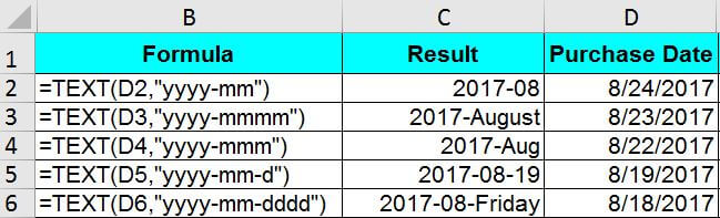
In this example, the first argument refers to a purchase date in Column C. The second argument is “format_text” and specifies how to display the result based on the format. Four ‘y’s as in ‘year’ display the year, and two ‘m’s as in ‘month’ display the month in two digits.
If you change it to four ‘m’s, it displays the month in English and if changed to three ‘m’s, it displays the month in three letters. Also, if you add one ‘d’ as in ‘day’, it displays the day. Changing it to 4 ‘d’s displays the weekday in English.
If you don’t use English on your computer, you may see something differently. There is a solution for that. Each language has a language code and putting the code at the beginning in the ‘format_text’ displays it properly. I’ll show you that. The language codes are 409 for English, 40a for Spanish, 439 for Hindi, 43e for Malay, etc. Put them in this format that you’re seeing.

By the way, you may have wondered how this TEXT function can actually be useful. In fact, it can be used to aggregate data by year or weekday, and many other ways. My company is a foodservice company. I often use this TEXT function to compare sales between weekdays.
This TEXT function can change not only the date but also other numerical values to displays various formats. For details, please refer to Excel Help. This is very handy function of Excel. While connecting to the Internet, press the ‘F1’ key on your keyboard to bring up Excel Help and you can search detailed explanations easily. Whenever you have a question, click the ‘F1’ key.
TEXT function can make your data analysis more meaningful to your readers
Lastly, I’ll show you examples of how I often use this TEXT function. I often see others’ data analysis only showing numbers and missing a solid conclusion. When you want to highlight your conclusion and add a little explanation, this TEXT function is a must to use.
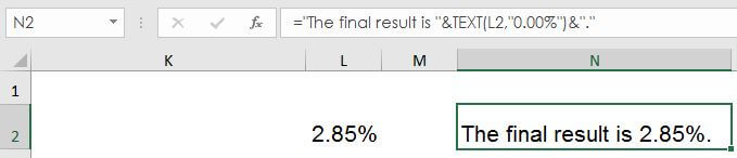
For example, let’s say that 2.85% is the final result of a data analysis. If it says “The final result is 2.85%.” near the result, it will be easier for my readers to understand my conclusion. Let’s do it here.
Type ‘=’ and ‘The final result is’, then it becomes an error. There is a rule that when enclosing a text in a formula, it has to be surrounded by double quotation marks. Therefore, put double quotation marks around the text, then it will show properly.
Next, in order to connect the result of Cell L2, you can use an ‘&’ mark. Put an ‘&’ and select the 2.85% cell, then you can connect them. However, it shows 0.0285 without the ‘%’ sign. Excel treats % as a format. Here the TEXT function is in play.

After the ‘&’ mark, type TEXT and ‘(‘ (parenthesis). After the ‘L2’, add a ‘,’ (comma). Then, ‘format_text’ becomes in bold. The format_text of % is “0.00%”. You can change its decimal by changing the number of ‘0’s. Then, close the parentheses and % appears now. However, I should have put a space after ‘is’, so I’ll do so. Lastly, add another ‘&’ and double quotation and ‘.’ (period) and another double quotation. Now it looks great.
By using this TEXT function, you can make your data analysis more meaningful to your readers. Please use this many times to master it.