Excel’s Conditional Formatting and Multiple Conditions【Excel Skill】
A situation where it’s easy to find the best next actions is called ‘Actionable’. You can make your data analysis actionable very easily with this Conditional Formatting. This article explains the basics of Conditional Formatting, how to use a conditional formula and how to write multiple conditions, step-by-step.
(Duration: 9:33)
<< Related Posts >>
- What is the basic of data analysis? That’s the PDCA Cycle! (DMAIC: Analyze Phase)
- Excel Absolute and Relative Cell References and Autofill Function【Data Analysis Excel Skill】
- Make your data analyses actionable all the time.
- The Basics of Conditional Formatting
- The ‘Duplicate Values’ function to make sure that there are no duplicate values.
- How to write a Conditional Formula
- ‘Absolute and Relative Cell References’ in Conditional Formatting
- How to write Multiple Conditions
Make your data analyses actionable all the time.
Hi, this is Mike Negami, Lean Sigma Black Belt.
Recently one of my friends asked me a question about Excel’s Conditional Formatting. By the way, if you have any questions or video requests, please write them in the comment section below.
The image above is a simple data analysis example. In the left table, the numbers are just lined up. On the other hand, in the right table, by using Conditional Formatting, customers whose ‘Gross Profit Increase’ (Column M) are below 0, are highlighted in pink. This helps us to find the next action to take. This is called making a data analysis ‘Actionable’.
There is always a purpose in data analysis. You should clarify it and make your data analyses actionable all the time. I made a video earlier about this topic. Please click on the link below and watch the video.
The Basics of Conditional Formatting
You can make your data analysis actionable very easily with this Conditional Formatting. If you haven’t used it until now, you are missing some low-hanging fruit. Please start using it today.
This example shows customers’ Sales, Gross Profit, and Gross Profit Increase for the last two months. We would like to find customers with a declining Gross Profit and take countermeasures quickly. Let’s walk through this and set the Conditional Formatting to highlight the cells whose increases are less than 0.
First select the range of cells where you want the Conditional Formatting, then select ‘Home’, ‘Conditional Formatting’ and ‘Highlight Cells Rules’ and ‘Less Than’. (See the image below.)
On the next screen, enter ‘0’ and click ‘OK’, then it’s done. Conditional Formatting can be used so easily.
This Excel version is Excel 2016, but if you use 2007 or newer, this process is almost the same.
These ‘Data Bars’ are also very useful. For example, let’s select the This Month’s Sales column in Column D and choose any favorite color of ‘Data Bars’, then you can visualize the differences in the sales among the others very easily. (See the image below.)
The ‘Duplicate Values’ function to make sure that there are no duplicate values.
As you can see, there are many kinds of ‘Conditioning’ and various ‘Formatting’. Which one do you think I use the most?
This one, ‘Duplicate Values’. This will highlight all duplicated-value cells within the selected range. In practice I often use it when there are many rows of data and I want to make sure that there are no duplicate values. Just select a range and choose ‘Duplicate Values’ and click ‘OK’.
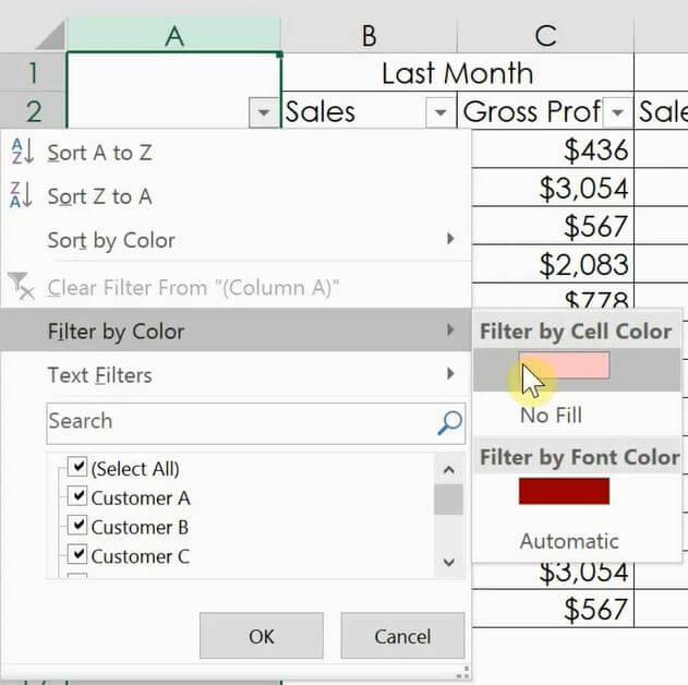
Click that column’s Auto Filter and see ‘Filter by Color’. If there is no pink color there, there are no duplicate values. If a pink color shows and you select it, you can easily see which values are duplicated.
How to write a Conditional Formula
Until now, the cells that the conditions refer to and the cells that you put formatting in were the same. Now, if you want to change the formatting based on other-cell values, how could you do it? In practice, you’ll have this case more often.
Suppose you want to highlight entire rows up to the customer names with the same condition as in the previous example. First let’s delete the conditional formatting we made. Select the cell you’ve set it in and from ‘Conditional Formatting’, choose ‘Manage Rules’. Your previous formatting is recorded. Select it and click ‘Delete Rule’, then click ‘OK’. It’s now deleted.
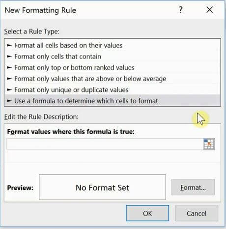
Select all the columns in the table and choose ‘New Rule’. There are many types of rules, but I always use this one: ‘Use a formula to determine which cells to format’.
Put a formula in the text box above for ‘What condition’ and set ‘What formatting’ you want in the below section separately.
At first, always put an ‘=‘ in the conditional formula. My condition of ‘Gross Profit Increase’ in Column F is below 0. Since F3 is the top row in the selected range, enter ‘=F3<0’.
Then click ‘Format’ to set what formatting you want to set when your condition is met. In addition to the previous ‘pink’ fill, you can change the ‘Number’ format, the style and color of the ‘Font’ and ‘Border’. In this example, click ‘Fill’ and choose any color you like, then ‘OK’ and ‘OK’.
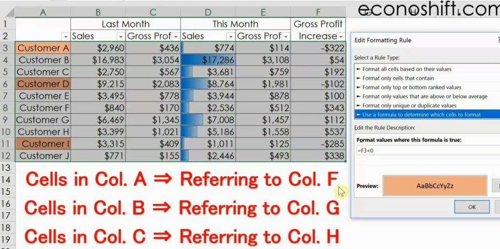
Lines from Column A to F are supposed to appear, but as the image above the result has not come out as I expected. This is because the conditional formula is not right. Let’s edit the Conditional Formatting we just made. Choose ‘Manage Rules’ and select it and click the ‘Edit Rule’ button, then you can go back to the same screen.
‘Absolute and Relative Cell References’ in Conditional Formatting
Here you need to use ‘Absolute and Relative Cell References’. I made a video about this, so if you are not familiar with it please watch the video first.
This ‘F3’ doesn’t have a dollar mark, so it’s treated as a Relative Reference. Since the selected range is from Columns A thru F, the conditions of the cells in Column A are referring to Column F, and when they are less than 0, the color appears properly.
However, The conditions of the cells in Column B refer to Column G and ones in Column C refer to Column H because they are Relative References. Since the referred cells are all blanks and the values are 0, they’re NOT below 0, therefore they don’t show the color.
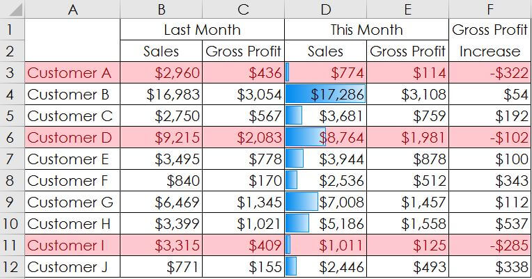
The solution is simple, and you only have to change the Relative References to Absolute References. Just put a $ mark in front of F in the conditional formulas. Please do not put a $ mark in front of the 3 because when you copy the cell and paste it below, you need Relative References. See the result. It went well. (See the image below.)
How to write Multiple Conditions
You can put Excel functions and multiple conditions in conditional formulas too. Suppose the two conditions are A and B. When you want your condition as ‘A and B’, you write ‘AND(A,B)’. If you want your condition as ‘A or B’, you write ‘OR(A,B)’.
For example, let’s add another condition that this month’s sales are 5,000 or more in addition to the previous condition. Put ‘AND(’ after the equal, and a ‘,’ after the previous condition. This month’s sales are in Column D and this should be an Absolute Reference, so put $D3 and put ‘>=5000’ and close the parenthesis. Press OK and OK.
Now only Customer D satisfied the two conditions. This means ‘the customer is large and the gross margin from them is declining. We need to deal with it immediately.’
The ‘Absolute and Relative Cell References’ in the 2nd half may have been difficult, but even if you only practice the contents in the first half, the quality of your data analysis will improve considerably, so please start using this Conditional Formatting from today.


